Model order reduction methods refer to a technique of applying surrogate models, also known as transfer functions or approximation models, to efficiently explore product design alternatives. Approximation models are highly effective, fast running mathematical models that are used in place of higher fidelity, long run-time simulation models typical with Finite Element Analysis (FEA), Computational Fluid Dynamics (CFD), and electromagnetic (EMAG) analysis. All simulation tools are approximations of reality. Reality involves physical testing under the conditions in which a product will be used. However, the cost and time of physical tests are usually time and cost prohibitive. Instead, simulation professionals use high fidelity simulation tools to replace or reduce physical testing.
Even with the compute power now available, the compute time and expense of these high-fidelity simulations can still be prohibitive, particularly when running Design of Experiments (DOE), Optimization, or Stochastic methods. Instead, model order reduction methods can be used to minimize the compute time and expense. These methods still require a valid sample data set to develop the mathematical model. A small sampling of the design space using the high-fidelity simulation tool driven by a Design of Experiments technique can be sufficient to create a reliable and accurate approximation model.
Dassault Systèmes’ SIMULIA Isight Solution
Isight provides designers, engineers, and researchers with an open system for integrating design and simulation models — created with various CAD, CAE, and other software applications — to automate the execution of simulations for design exploration and optimization. The software solution can easily create an approximation model for any task or individual application component, from any source of simulation or test result data. There are numerous benefits of using Isight to create approximation models:
- Deliver more reliable and robust products through accelerated evaluation of design alternatives
- Reduce design cycle time through integrated workflow processes
- Integrate models developed in popular commercial software and in-house developed codes
- Manipulate and map parametric data between process steps and multiple simulations to improve efficiency with fewer manual errors
- Check the accuracy of the model and automatically add additional data points to achieve the desired accuracy
Approximation Models Available in Isight
There are different types of approximations models. No one technique is best for all applications as the physics involved vary. The various types of approximation models available in Isight are described below:
Response Surface Models (RSM)
RSMs are polynomials up to 4th order with four Term Selection techniques. You can use Term Selection to remove some polynomial terms with low significance. This can improve reliability of the approximation and reduce the number of required design points.
- Sequential Replacement
- Stepwise Efroymson
- Two at a Time Replacement
- Exhaustive Search
Kriging
Kriging approximation is a type of interpolation technique. Kriging approximations are extremely flexible due to the wide range of correlation functions, which can be chosen for building the meta model. Furthermore, depending on the choice of the correlation function, the meta model can either “honor the data”, providing an exact interpolation of the data, or “smooth the data”, providing an inexact interpolation.
The Isight implementation of Kriging models allows the use of the common correlation functions such as Exponential, Gaussian, Matern Linear and Matern Cubic.
Initialization of the Kriging approximation requires at least 2n+1 design points, where n is the number of inputs. The component being approximated can be executed multiple times to collect the required data. Alternatively, a data file can serve as the initialization source.
Orthogonal Polynomial
Orthogonal Polynomial approximation is a type of regression technique. Orthogonal polynomials minimize the autocorrelation between the response values that exists because of the sampling location. Another advantage of using functions that are orthogonal with respect to the data is that the inputs can be decoupled in the analysis of variance (ANOVA).
Chebyshev orthogonal polynomials are a common type of orthogonal polynomials that are particularly useful for equally spaced sample points. They are used when the sampling strategy is an orthogonal array. Isight allows the use of Chebyshev polynomials even when other sampling strategies are used, in this case however, ANOVA cannot be computed.
Isight also provides the ability to generate Orthogonal Polynomial approximations for other kinds of sampling. The successive orthogonal polynomial technique generates a series of polynomials that are orthogonal with respect to the data provided. These polynomials are then used as basis functions to obtain an approximation for the responses. Note that the basis functions only depend on the sample locations and not the response values.
Initialization of the Orthogonal Polynomial approximation requires at least 2d+1 design points, where d is the degree of the expected polynomial. The data file must contain the required number of data points.
Radial Basis Function
Radial Basis Function (RBF) approximation is a type of neural network employing a hidden layer of radial units and an output layer of linear units. RBF approximations are characterized by reasonably fast training and reasonably compact networks. They are useful in approximating a wide range of nonlinear spaces.
Elliptical Basis Functions (EBFs) are similar to Radial Basis Function but use elliptical units in place of radial units. Compared to RBF, where all inputs are handled equally, EBF networks treat each input separately using individual weights.
RBF networks are characterized by reasonably fast training and reasonably compact networks. EBF networks, on the other hand, require more iterations in order to learn individual input weights and are often more accurate than RBFs.
Initialization of the RBF approximation requires at least 2n+1 design points to be evaluated, where n is the number of inputs. The component being approximated can be executed multiple times to collect the required data. Alternatively, a data file can serve as the initialization source.
Automatic Generation and Cross-Validation of Approximation Models
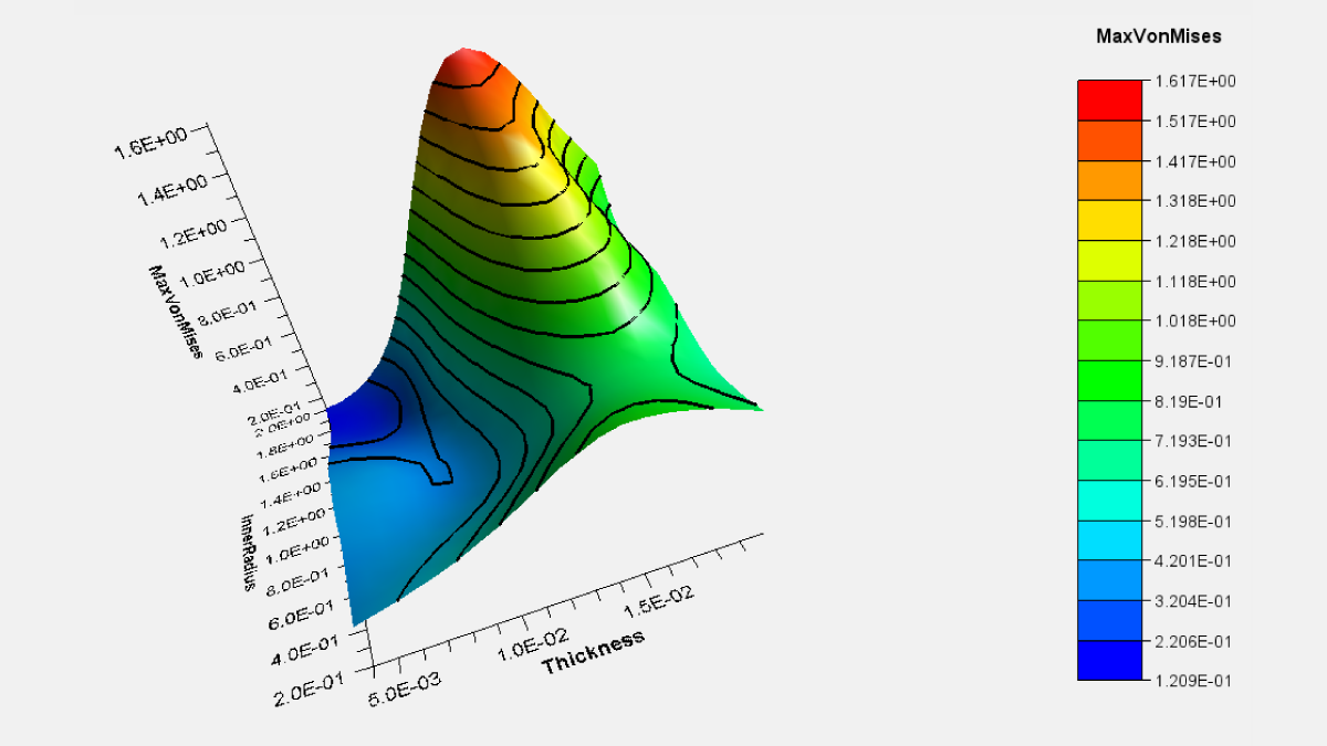
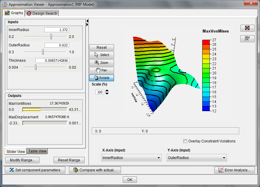
All model order reduction methods in Isight support automatic generation and cross-validation of approximation models with easy-to-understand visual error analysis. The approximation creator/viewer interface in Isight allows users to visualize approximation surfaces in 2D and 3D – see Figure 2 below.
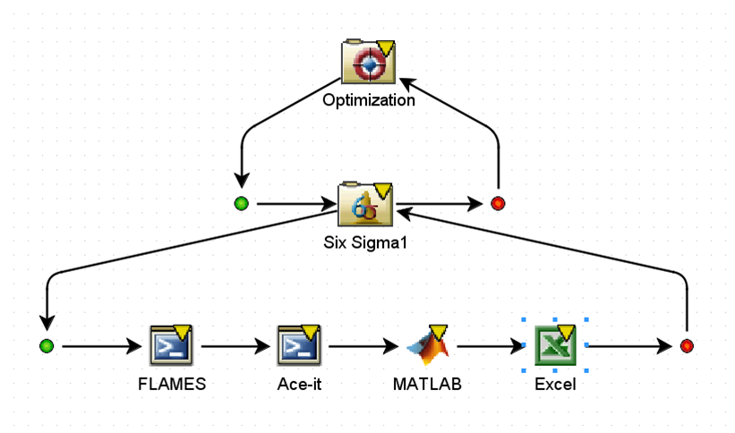
Shown below in Figure 3 is a typical Isight workflow that incorporates an approximation model. As noted above, an approximation can be dropped on an entire process, sub-process, individual component, or dropped on the workflow as a stand-alone component if the model had been previously saved or data exists to create the model. If the approximation model is dropped on a process, sub-process, or individual component and has no data for it to be initialized, Isight will automatically run the process until it gets the minimum number of points to initially create the approximation.
It will then automatically run an error analysis by running a design point with the approximation model and then running the simulation for which it is approximating. If the results between approximated and actual run differ by a specified percentage, Isight will continue to add more runs of the actual simulation to the approximation model until the error tolerance has been satisfied.

This automatic generation/initialization of an approximation model can be part of any design exploration technique: DOE, Optimization, Monte Carlo, Six Sigma, etc. The final “best” design from the approximation can then be automatically rerun with the actual simulation tool so you have the full simulation results of your tool of choice.
Questions?
If you have any questions or would like to learn more about how to work with approximation models in SIMULIA Isight, please contact us at (954) 442-5400 or submit an online inquiry.