The size and complexity of product designs that are analyzed and tested with Abaqus – a finite element analysis (FEA) and multi-physics engineering simulation software – continues to grow. Submodeling is an effective technique that can be used when detailed product simulation results are required for a small, localized region within a larger model, allowing the analyst to significantly reduce the computational demands and runtime of an analysis.
A global analysis of a structure can first be used to identify areas where the response to the loading is critical. A local submodel can then be created for the critical areas, with improved geometric representation and/or mesh refinement. This local submodel provides increased accuracy over the global model without the requirement to remesh and reanalyze the full model. This approach results in reduced analysis costs while maintaining sufficient details in critical regions.
In this blog, we will look at the theory behind submodeling, the two submodeling techniques available in Abaqus, and how to implement submodels. We will also highlight the limitations of submodeling in Abaqus and the important step of verifying analysis results.
Theory of Submodeling
Submodeling in Abaqus utilizes Saint-Venant’s Principle, whereby the boundary of the submodel is sufficiently far from the region of interest within the submodel to permit the applied forces being replaced with equivalent local forces. The global model solution is used to define the behavior of the submodel boundary through the control of driven variables that are representative of the applied forces. The solution in the area of interest is not changed by the end effects as long as the end loads remain statically equivalent.
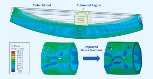
In Figure 1, an example of beam with several localized openings is shown. The global model of the full beam is used to determine the driven variables as output at the common boundaries for the submodel and facilitates the use of a relatively coarse mesh. Analyses are performed independently on the global model and submodel, with the driven variables being the only link between the two. With this independence there is flexibility to change geometric features, element types, material properties, etc. to improve the representation of the submodeled region. As with any modeling technique, it is important to validate the results to ensure they are physically meaningful. Comparison of contour plot near boundaries of the submodeled region of the global and submodel can be used to confirm the results are consistent.
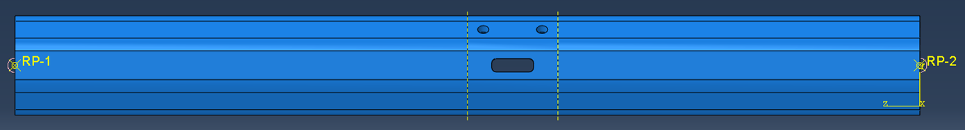
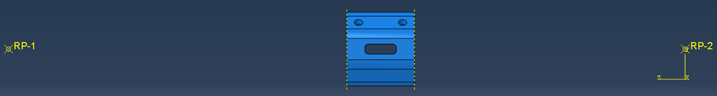
Figure 1: Global Model and Submodel
Submodeling Techniques in Abaqus
Within Abaqus there are two techniques are available for submodeling which are referred to as node-based and surface-based submodeling. The node-based technique interpolates the nodal results field from the global model onto submodel nodes, this is the more general and commonly used technique. Conversely, in surface-based submodeling the stress field is interpolated onto the submodel surface integration points. Surface-based submodeling is limited to solid-to-solid applications and static analysis, for all other purposes node-based submodeling should be applied. Either technique, or a combination of the two can be used within an analysis depending on the attributes of the model.
The surface-based technique can provide more accurate stress results if in a static analysis if there is a significant difference in the average stiffness in the region of the submodel and the global model is subject to force-controlled loading. Whereas, when the stiffness in the regions is comparable, node-based submodeling will provide similar results to surface-based submodeling with reduced potential for numerical issues caused by rigid-body modes. Differences in stiffness may occur as a result of additional detail in the submodel such as openings or fillets, or from minor geometric changes which do not warrant re-running the global analysis.
If the model is subjected to large displacements or rotations node-based submodeling can improve the accuracy when transmitting large displacements and rotations to the submodel. Depending on the output results that are of greatest interest. Node-based submodeling will provide a more accurate transmission of the displacement field in the submodel. Whereas surface-based submodeling will provide a more accurate transmission of the stress field, resulting in more accurate determination of reaction forces in the submodel. The two techniques can be included within a single model at different boundaries.
Implementing Abaqus Submodels
The local model can be driven using data saved to the output database file (in ODB or SIM format). Node-based submodels can also be driven using the results (.fil) file. Only those variables written to the output database will be used in the submodel, so it is important to save adequate output data at sufficient frequency. These results must be saved in the global coordinate system for interpolation onto the submodel. In the case of nodal data, values are always written with respect to global directions to the output database file, regardless of whether nodal coordinate transformations are used. All driven variables should be saved at a common frequency during the global analysis, and this frequency should be sufficiently fine to allow adequate reproduction of the global time history for the driven variables. If the results are saved at different frequencies, the coarsest frequency will be used in the submodel analysis. It is recommended that you create a single set containing all the node sets and/or element sets from which to drive the submodel. In Figure 2, the set defining the submodel boundary is highlighted in red and is labeled as Submodel-Region.
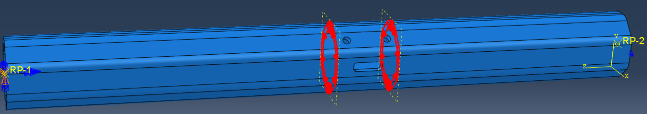
Figure 2: Submodel Boundary
All types of loading and prescribed boundary conditions can be applied to the submodel. However, care should be taken to apply loads and boundary conditions in the submodel in a manner that is consistent with the global model to avoid incorrect results. Only the driven variables will be interpolated and transferred to the submodel. Any predefined fields must be provided as they were in the global model. Initial conditions should be consistent between the global model and the submodel. For simplicity, it can be helpful to copy the initial global model to create the submodel (Figure 3), using the create cut tools to remove material outside of the submodel boundaries as shown in Figure 4. This approach will allow retention of the global model settings and minimize the potential for errors in creating the submodel.
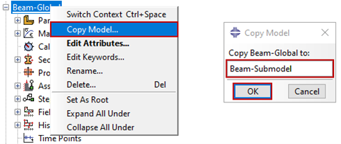
Figure 3: Copy Global Model to Create Submodel
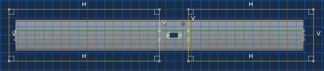
Figure 4: Cut Geometry
The step time in the submodel analysis should match the step time in the global analysis or any interpolation with respect to time will be incorrect. If there is any discrepancy, the time period of the global step can be scaled to that of the submodel by toggling on the option to Scale time period of global step to time period of submodel step when implementing the boundary conditions shown in Figure 5.
Driven nodes are defined through the submodel boundary conditions. You may specify which degrees of freedom are to be driven at the boundary of the submodel – typically all degrees of freedom at the driven nodes are specified. In addition to scaling the time period, Abaqus can scale the value of driven variables applied to the submodel from the global model when appropriate. In Figure 5, a submodel boundary condition is implemented and includes all degrees of freedom available for solid continuum elements (1-3) with no scaling. Note that only the fundamental solution variables can be driven. In either solid-to-solid or shell-to-shell submodeling this includes displacements, temperatures, electric potential, pore pressure, etc. Velocities or accelerations on the submodel boundary cannot be driven. Abaqus selects the driven variables automatically when a global shell model is used to drive a local solid model. Other submodel boundary conditions can be created, modified, or removed as usual.
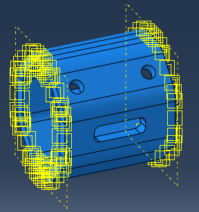
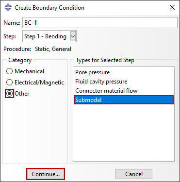
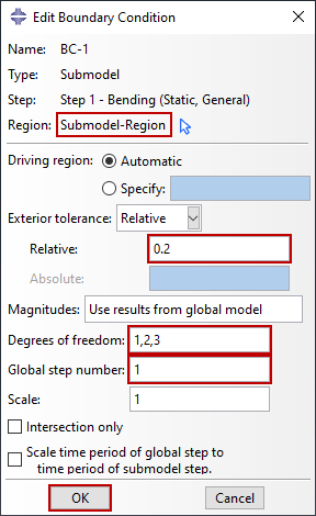
Figure 5: Submodel Boundary Condition
Abaqus interpolates in both space and time to determine the values of the driven nodal variables throughout the step of the submodel analysis. The order of spatial interpolation of the driven variables is dictated by the order of elements used at the global level. Automatic time incrementation is applied independently in the global and submodel analyses. Independent time incrementation is accommodated by the temporal interpolation of the driven variables. Linear temporal interpolation is used between the values read from the output database or results file.
When the global model undergoes large displacements or rotations, the user must ensure that the submodel also undergoes these displacements or rotations. When node-based submodeling is used, the driving nodes automatically account for displacements and rotations so the submodel will be correctly positioned relative to the global coordinate system. Conversely, for surface based submodeling, using only surface tractions provides the submodel with no displacement information. Instead, to account for the displacements, the submodel must include: applied boundary conditions, driven nodes, and inertial relief. When both methods are used it is important to maintain a consistent driving method across the selected area to prevent overconstraints arising from partial or excessive driving definitions.
When setting up a submodel the model attributes should be modified to refer to the output database or results file. The model attributes shown in Figure 6 would cause Abaqus to read the Beam-Global.odb output database file and use those results in an analysis of a submodel defined in the Beam-Submodel.inp input file.
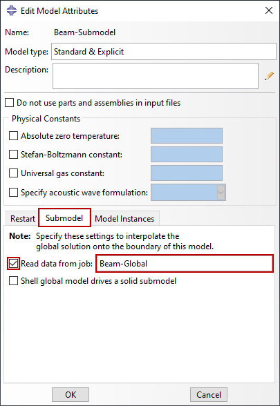
Figure 6: Submodel Attributes
Limitations of Submodeling
There are some limitations on the methods and element types that are compatible with the submodeling approach. Limitations will be briefly outlined here with more information on these to be found in the documentation.
Elements that can be used at the global and submodel levels are limited to first and second-order triangular and quadrilateral continuum, shell, or membrane elements, first and second order tetrahedral, wedge, or brick continuum elements. Global models can contain both solid and shell elements, with the condition that all driven nodes must lie within the shell elements in the global model.
The submodel boundary nodes cannot lie in regions of the global model where there is insufficient information for interpolation of the driven variable. This includes regions where there are only one-dimensional elements (such as beams, trusses, links, or axisymmetric shells), user elements, substructures, springs, dashpots, other special elements, or axisymmetric elements.
When using shell elements, five degrees of freedom per node shell elements (S4R5, S8R5, etc.) should typically be avoided at the global level as the rotations are not saved. These elements cannot be used in shell-to-solid submodeling.
Submodels cannot be used in coupled thermal-electrical, coupled thermal-electrochemical, and mode-based linear dynamics procedures. Surface-based submodeling can only be used in general static procedures. Shell-to-solid submodeling cannot be used with any other type of submodeling in the same model.
Verification of Analysis Results
When using the submodeling approach, two sets of analysis results are subsequently obtained: the first from a global model giving an approximation of the behavior, and the second from a refined local model giving more precise representation of detailed output. An important step in the submodeling procedure is verification of the results. In Figure 7, the results of a node-based submodel are shown. The model is first checked for consistency of displacements in the region of the submodel prior to plotting the stress gradient. If major discrepancies are identified with the displacements, this will affect all subsequent results and the model should be reviewed and resubmitted. Once the displacements are found to match, other output such as stresses can be interrogated. Here an improvement is the stress gradient is achieved by increasing the mesh density in the submodeled region. Stresses in other regions of the beam can be obtained from the global model where, in the absence of stress concentrating openings, the coarse mesh is sufficient.
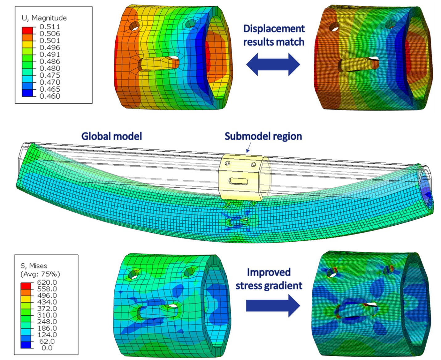
Figure 7: Results Verification
Questions?
If you have any questions or would like to learn more about submodeling in Abaqus, please contact us at (954) 442-5400 or submit an online inquiry.