For many additive and subtractive processes in construction and manufacturing, finite element analysis (FEA) can effectively be used to understand the impact of adding or removing material. Such as concrete, plastic, metal, and more. FEA increases the precision of calculations and reduces prototyping demands by enabling users to virtually evaluate the effects of heat transfer, changes to self-weight, or other loading scenarios associated with these processes, to assess the resulting displaced shape, stress state, potential cracking, and part distortion. Material within a digital model can be added or removed instantaneously. Or, subject to gradual material changes, to guide suitable material selection and process optimization before physical investments are made.
Material Addition & Removal in Construction & Manufacturing
The addition of material is used in construction and manufacturing processes. Slip form concrete construction and roller compacted concrete are placed in lifts where material is added sequentially to the structure. Heat is released as a byproduct of concrete curing, inducing thermal stresses that can cause cracking. The additional mass contributed by the new material will be carried by concrete that is itself curing and gaining strength. This process parallels that of additive manufacturing. Although the scale and materials vary, the modeling process to assess material addition impact is consistent. Welding is a subset of this, involving high temperature and progressive material addition.
The inverse of this is the removal of material in physical, chemical, or other machining processes. Techniques used to remove material produce heat that is transferred to the material that remains. The resulting thermal expansion can cause a combination of temporary and permanent distortions. And, the amount of material to be removed should account for the eventual contraction and possible distortion of the part.
How to Use Abaqus to Virtually Assess and Optimize Material Addition & Removal
SIMULIA Abaqus software provides several options to simulate the removal or addition of material; change of state, material field variables, and progressive element activation. Contact activation/deactivation may be used independently or together with the different approaches available and in Abaqus 2022, this functionality was extended to general contact in Abaqus Standard. In this blog post, we will look at how to apply change of state and material field variables within Abaqus/Standard.
Change of state permits elements to be deactivated or activated within a step, while field variables can be used to change material properties to mimic the effect of removal or addition. Field variables can be favorable when a gradual increase or decrease in stiffness is needed as opposed to an instantaneous change of state. These procedures can be applied independently or in tandem to achieve the desired result. Progressive element activation is a higher fidelity method, permitting both full and partial element activation. More information on this method can be found in the Abaqus documentation.
Model Setup
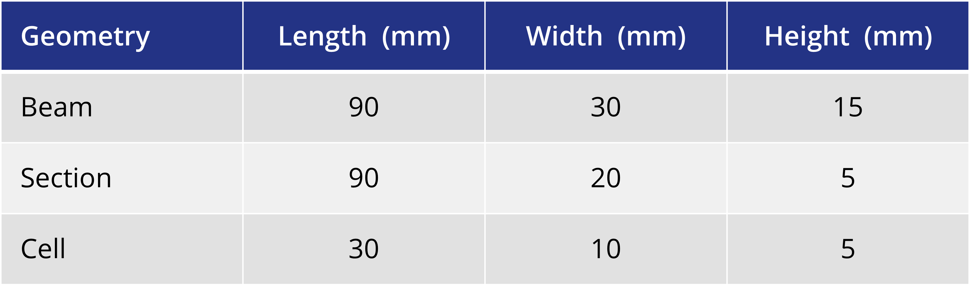
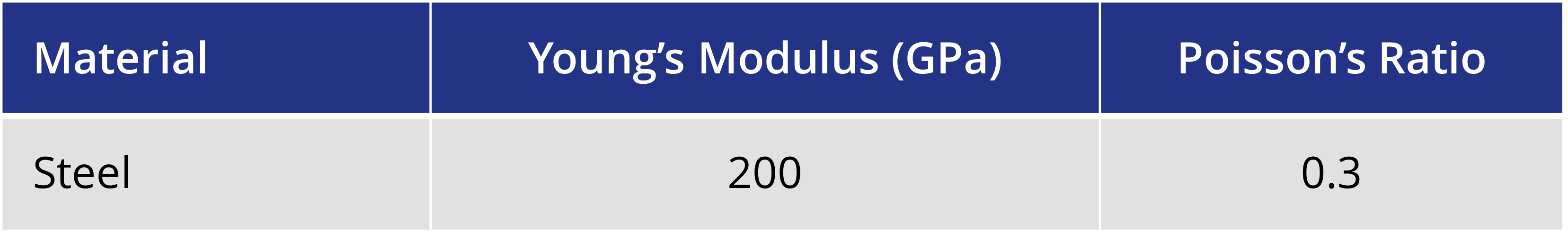
Illustrative examples will be used to explain these processes, as the field variables and model change methods will be used to achieve the same result. These examples will focus on the context of stress/displacement elements; however, the methods can be applied more broadly. A rectangular part will have a section removed segmentally as eight cells. The geometric properties are given in Table 1 and material properties in Table 2.
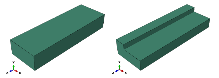
The initial and final geometry is shown in Figure 1. The part is transitioned from the initial to final configuration by individually removing or degrading eight cells within the part.
Regardless of the method selected, the first step in this procedure is partitioning of the geometry to establish the cells identified for removal. The part geometry should reflect the maximum size – if material is being removed, this will reflect the initial geometry; and if material is being added, this will reflect the final geometry. By partitioning the part, individual sets can be assigned to the cells being removed.
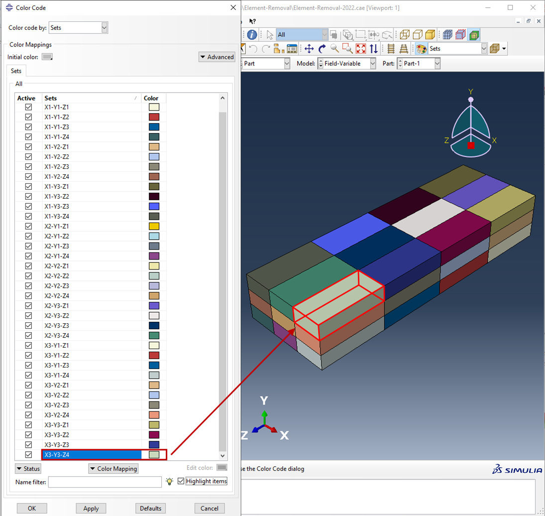
For this example, the part geometry is partitioned into 3 × 3 × 4 cells as shown in Figure 2. Sets are then assigned to the individual cells based on the geometry at the part level. This approach is robust when remeshing is required and the sets are accessed within the assembly as partname-instance.setname. Here the sets have been named based on their x,y,z position within the part form X1-Y1-Z1 to X3-Y3-Z4 – the later part is highlighted in Figure 2. The part name is Part-1 and the first and only instance of this part is labeled Part-1-1. Set X3-Y3-Z4 is subsequently identified as Part-1-1.X3-Y3-Z4 at the assembly level.
Field Variables
Spatial variation of field variables is used to initiate local material degradation, and subsequently the effect of material removal or addition. The material properties are written with a dependency on assigned field variables. Temperature dependency is a specific example of this general framework. By changing the value of the field variable within a step, the properties are altered at an assigned time within the simulation. Amplitudes are tied to the field variables for the required sets to manage the spatial variations and subsequently control which cells are subjected to a change in material properties. In this example, Young’s modulus and Poisson’s ratio are degraded to the point of having a negligible effect on the stiffness of the part for eight cells within the model.
In Figure 3, the material properties with field variable dependencies are shown. The number of field variables is set to 1. When Field 1 equals 1, Young’s modulus value is 200 000 MPa and Poisson’s ratio is 0.3. When the Field 1 value increases to 2, these properties are decreased to 2 MPa and 0.01 respectively, which can be considered negligible.

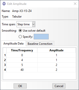
One or more amplitudes are determine to introduce spatial variability of field variables and manage the removal of elements over the time step. A unique amplitude is set for each of the eight cells being removed and the removals are staggered by varying the tabulated values. In Figure 4, the tabular Amplitude relative with set X3-Y3-Z4 is shown. The field variable associated with the amplitude will increase from 1 to 2 at a step time of 4, and remain equal to 2 until the end of the step. This is the fourth set to be degraded in the step, and a total step time of 8 seconds is used to degrade each set individually
One or more amThe amplitudes are tied to the unique sets by making modifications to the model in the keyword editor found at Model -> Edit Keywords -> ModelName.
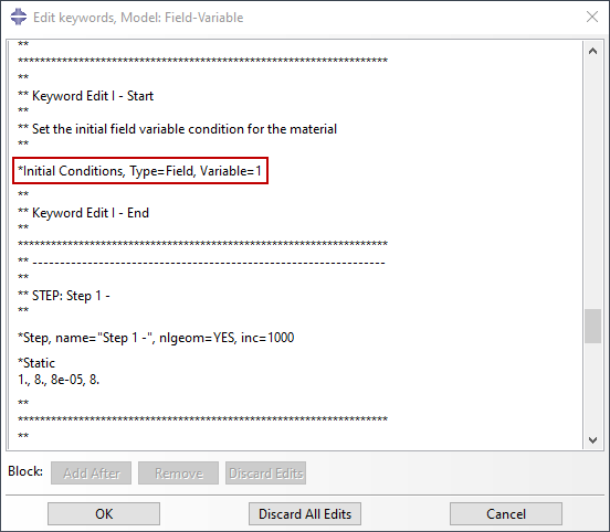
An initial condition is set with the field variable equal to 1 prior to Step 1 as shown in Figure 5.
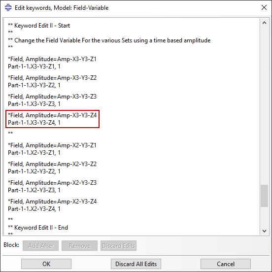
In the desired step, change the field variable according to the time-based amplitude. Here the amplitude function Amp-X3-Y3-Z4 is linked with the set Part-1-1.X3-Y3-Z4 on the assembly level and field variable 1, as shown in Figure 6.
By defining a material with field variable dependencies, writing multiple amplitude functions, and associating each amplitude function with the field variable and a unique set within the model. It is possible to vary the material properties at different locations through the analysis. We rapidly reduce the properties to mimic the effect of material removal. But, the inverse would be possible for material addition. Additionally, if a material strength curve is established the amplitude function could be used to define a gradual increase or decrease in strength with time. Aging of elastomers is degradation over loading, temperatures with time. When using this technique, care should be taken in applying boundary conditions and loads. This is to avoid element distortion where the material properties have been degraded.
Model Change
The model change type interaction is to initiate the addition or removal of a model region during a step. Upon removal, Abaqus/Standard stores the forces/fluxes that the region had exerted on the remaining parts of the model at the nodes on the boundary between them. Over the removal step, these forces are ramped down to zero. Which ensures a smooth effect on the model that does not impede convergence. If there is model change is for the addition of material, the initial step will be on what is effectively the final geometry. The cells that will be added to the model should be removed using a model change interaction in the first step, then individual cells can be added as required in subsequent steps. Two types of reactivations are provided for stress/displacement elements: strain-free reactivation and reactivation with strain. Further information on these options is available in the Abaqus documentation.
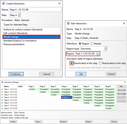
The removal of cells using a model change interaction is shown in a second model. In Figure 5, a model change Interaction set for X3-Y3-Z4. As was done for the use of field variables, this set is the fourth we remove from the model. To achieve sequential removal, set X3-Y3-Z4 is subsequently deactivated in Step-4. For simultaneous removal of multiple cells, alternate sets could be defined containing all required cells. In the Edit interaction dialog box, the geometry region is selected by set for the set named Part-1-1.X3-Y3-Z4. Other region types we can select for removal/addition are Skins, Stringers, or Elements. The option to Deactivate is on by default as deactivation must occur prior to reactivation in a model change analysis.
Material removal/addition may cause numerical problems and requires special attention. To avoid these issues and other common problems use the following guidelines:
- Boundary Conditions: Removal of material in a static stress analysis. It is important to ensure that the remainder of the model is sufficiently constrained to prevent an unconstrained rigid body mode.
- Loads: Distributed and concentrated loads applied in areas where elements are removed or reactivated may require modification.
- Elements: Support removal in not currently available for rigid, cohesive, gasket, and piezoelectric elements. Removal and reactivation of all other element types in Abaqus/Standard is accessible.
- Contact: If elements that are connected to a contact pair are removed, the contact pair should be removed or deactivated when model change is initiated.
- Constraints: If all elements attached to a node constrained with a multi-point constraint or a linear constraint equation are being removed, this node should be the dependent node of the multi-point constraint or linear constraint equation.
- Warnings: In some cases, element removal may cause Abaqus/Standard to report extra unconnected regions in the message file. It is safe to ignore these messages.
In this example, use of the model change interaction is to individually remove each set from the assembly. For sequential removal, each set is in a separate time step, and care is taken to ensure loads and boundary conditions impacted by the removal are subsequently adjusted, avoiding rigid body motion. In the case of material addition, the material being added will first be removed, then added back to the model when appropriate. You can add field variable dependencies to models containing model change interactions depending on the simulation needs.
Questions?
If you have any questions or would like to learn more about how to use Abaqus simulation to understand the effects of additive and subtractive processes, please contact us at (954) 442-5400 or submit an online inquiry.