Abaqus provides capabilities of modeling composite structures in different ways. Depending on the type of composite being modeled, material data available, boundary conditions and also the desired results, a particular approach may work better than other. This blog article tries to summarize the methods available and focuses on a specific modeling approach to model composite laminates.
What is a composite structure anyway?
A composite is a macroscopic mixture of a reinforcement material embedded inside a matrix material. A composite structure is made of a composite material and could have many forms like a unidirectional fiber composite, a woven fabric or a honeycomb structure.
Abaqus uses several different methods to model composite structures [1]
1) Microscopic: In this approach, matrix and reinforcements are modeled as separate deformable continua
2) Macroscopic: In this approach, matrix and reinforcements are modeled as separate deformable continua. This approach could be used when microscopic behavior of individual fibers and their interaction with the matrix are of importance.
3) Mixed modeling: In this approach, the composite structure is modeled as a single orthotropic (or anisotropic) material. This is important when the global behavior of the structure is more important than its behavior at microscopic level. A single material definition (often anisotropic) is sufficeent to predict the global behavior.
 Analysis of a composite laminate:
A composite laminate is made of multiple layers. Each layer, also referred to as a ply, has a unique thickness and reinforcement fibers in each layer are aligned differently. The sequence in which the plies are arranged to form the laminate is called a layup or a stacking sequence. The easiest way to model this in Abaqus is using a mixed modeling approach. This will consist of defining for each ply, an orthotropic property, thickness, fiber orientation and the stacking sequence which would in turn govern its structural behavior.
Often, laminate properties are directly obtained from experiments or from other applications. These properties could be in the form of A, B, D matrices which define the stiffness of the laminate. In such situations, macroscopic approach could be used for structural analysis of the laminate. This approach presented could be considered macroscopic in nature as equivalent section properties are derived and used in Abaqus section definition. It can also be argued that it is a mixed modeling approach as the sectional stiffness is derived based on a ply layup.
Following example shows how the A, B, D matrices are derived from the available layup information and used in a General Shell Section definition in Abaqus.
Assumptions of Classical Lamination Theory:
Macroscopic modeling approach for laminated composites shown here, is based on the Classical Lamination Theory (CLT). For accurate implementation of CLT following assumptions need to hold true [2]:
• The displacement components through the thickness of the laminate are continuous and there is no slip between adjacent plies of the laminate.
• Each ply is in a state of plane stress.
• The laminate deforms such that the straight lines normal to the mid-plane, remain straight & normal to the mid-plane after deformation and the thickness of the plate does not change due to deformation
Example:
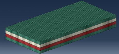
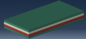
A composite panel consists of 2 layers (plies) of unidirectional graphite fibers in an epoxy resin (Figure 1). Each layer is 0.1mm thick and the orthotropic material properties for both the layers are as follows:
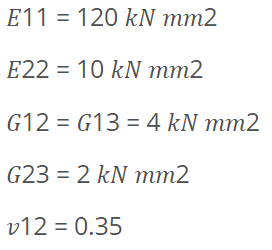
Here, the direction 1 refers to longitudinal (along the fiber), 2 refers to transverse (perpendicular to the fiber in the plane of the lamina) and 3 refers to the direction normal to the lamina. Thus, these directions are local to the ply.
In order to use this approach, stacking sequence of the plies needs to be known. The stacking sequence in this example is {0/90} which means that the fibers in first layer are oriented in a direction perpendicular to the fibers in the second layer. Let the first layer have fibers oriented along global X axis and the second layer have fibers oriented along global Y axis.
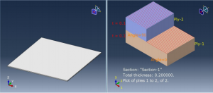
Figure 1
Assuming a state of plane stress in each ply, the resultant stresses are related to generalized strains using following equations:
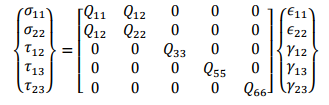
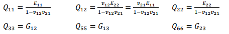
The stiffness terms in above equation are related to the usual engineering constants of an orthotropic material by the following relations:
These are the local stiffness terms for each ply along the principal ply directions. As the principal directions in every ply are different, the local stiffness components computed above for each ply, need to be rotated to a system (1, 2, ????) that refers to the standard shell basis directions chosen by Abaqus by default. This can be achieved by a coordinate system transformation and leads to the following relations:
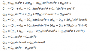
Thus, ????̅ ???????? terms are the stiffness coefficients along standard shell basis directions.
The equivalent sectional stiffness can then be defined based on these stiffness coefficients and the geometric configuration of the laminate. This leads to the following three matrices:
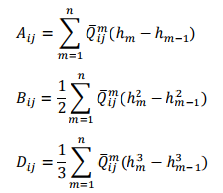
Here ???? indicates a particular layer. Thus, ????̅ ???????? ???? depends on the material properties and fiber orientation of the ????????ℎ layer.
ℎ???? and ℎ????−1 in these equations indicate that the ????????ℎ lamina is bounded by surfaces ???? = ℎ???? and ???? = ℎ????−1 and ℎ????is the distance of the ????????ℎ lamina from the midplane of the laminate. This nomenclature is shown in the figure below:
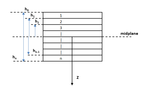
Figure 2
The resultant ????,????, ???? matrices provide the general laminate stiffness and have a very important consequence as such. ???? matrix is the normal matrix and its terms relate the normal stresses and strains. The ???? matrix is a coupling matrix and it relates the bending strains with normal stresses and normal strains with bending stresses. The third matrix is called the ???? matrix and its terms relate the bending strains and stresses. Please note that the transverse shear stiffness terms could also be computed from underlying equations, but are ignored for this particular example.
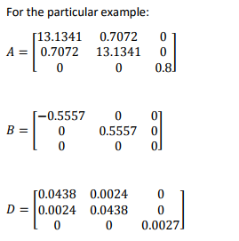
These A, B and D matrices could be combined and used directly in a general shell section definition in Abaqus:
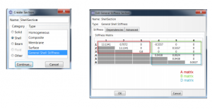
The A, B, D matrices are very important as they provide a direct relationship between the laminate forces and moments on the shell section (membrane forces per unit length, bending moments per unit length) {????} and the laminate generalized section strains (reference surface strains and curvatures) {????}.
{N} = [D]:{E}
Also, these matrices can be used to determine the in-plane engineering constants which could further be used for structural analysis of the composites.
References:
Abaqus Example Problems guide: 1.2.2 Laminated composite shells: buckling of a cylindrical panel with a circular hole
[1] Analysis of Composite Materials with Abaqus course
[2] Composite Materials and Structures, Dr. P. M. Mohite, Module 5, Lecture 16: Introduction to classical plate theory (http://nptel.ac.in/courses/101104010/)